Radial Basis Function Network(RBFN)

Radial basis function network can be used for approximating function and recognizing patterns. It uses Gaussian Potential functions.

Architecture

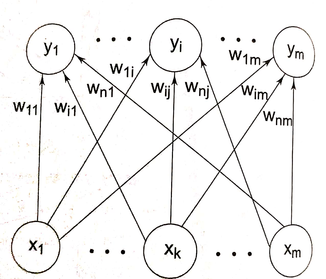
The architecture radial basis function network consists of three layers, the input,hidden and the output layer as shown in below figure. The architecture of RBFN is a multi layer feed forward network. There exist ‘n’ number of input neuron and ‘m’ number of output neurons with the hidden layer existing between the input and output layer. The interconnection between the input layer and hidden layer forms hypothetical connection and between the hidden and output layer forms weighted connections. The training algorithm is used for updation of weights in all the interconnections.

Training algorithm for RBFN

The training algorithm for the radial basis function network is given below.  Radial basis function uses Gaussian activation function. The response of such function is non-negative for all value of x. The function is defined as, f(x)=exp(-x²)

Step 1: Initialize the weights (set to small random values)

Step 2: While stopping is false do step 3-10

Step 3: For each input do steps 4 – 9

Step 4: Each input unit (x_i ,i=1,2.....n) receives input signal to all unit in the layer above(hidden unit)

Step 5: Calculate the radial basis function

Step 6: Choose the centres for the radial basis functions. The centres are chosen from the  set of input vectors. A sufficient number of centers have to be selected in order to ensure adequate sampling of the input vector space.

Step 7: The output of i_m unit v_i(x_i) in the hidden layer.      

$$ v_i(x_i)=exp(-\sum_{j=1}^r[{{x_{ji}-\bar{x}_{ji}]^2}\over{\sigma^2_i}}) $$
Where $\bar x_{ji}$ = Centre of the RBF unit for input variables
$\sigma _i$ = Width of the RBF unit
$x_{ji}$ = $j_{th}$ variable of unit pattern

Step 8: Initialize the weights in the output layer of the network to some small random value.

Step 9: Calculate the output of the neural network
$$ y_{net}=e\sum_{i=1}^Hw_{im}v_i(x_i)+w_0$$
Where, H = Number of hidden layer nodes(RBF function)
$y_{net}$ = Output value of the $m_{th}$ mode in output layer for the $n_{th}$ incoming pattern.
$w_{im}$ = Weight between  $i_{th}$ RBF unit and  $m_{th}$ output node
$w_0$ = Biasing term at $n_{th}$ output node

Step 10: calculate error and test stopping condition.

The stopping condition may be the weight change, number of epochs, etc.             

Learning Vector Quantization(LVQ)

Vector quantization is a standard statistical clustering technique, which seeks to divide input space into areas that are assigned as "code book" vectors. In LVQ network, target values are for the input training pattern and the learning is supervised. In training process, the output units are positioned to approximate the decision surfaces. After training, an LVQ net classifies an input vector by assigning in to same class as the output unit that has its weight vector(reference or code book vector) closest to input vector.

In order t understand the LVQ techniques , it should be borne in mind that the closest weight vector Wj to pattern X may be associated with a node j, that has the wrong class label for X. This follows because the initial node labels are based only on their most frequent class use and are therefore not always reliable. The procedure for updating wj is given by,

                       1. if x is classified correctly, ∆W_j=α[x-w_j]

                       2. if x is classified incorrectly, ∆W_j=-α[x-w_j]

The negative sign in the misclassification makes the weight vector move away from the cluster containing x, which, on average, trends to make weight vectors move away from the boundaries.

Architecture

The architecture is shown in below figure. The architecture is similar to the architecture of SOM without a topological structure assumed for the output units. in LVQ net, each output unit has a known class since it is supervised learning, thus differs from SOM which uses unsupervised learning. 

Training Algorithm

The  algorithm for the LVQ net is to find the output unit that has a matching pattern with the input vector. At the end of the process, if x and w belong to the same class, weights are moved toward the new input vector and if they belong to a different class, the weights are moved away from the input vector. In this case also similar to SOM, the winner unit is identified. The winner unit index is compared with the target, and based upon its comparison result, the weight updation is performed as shown in the algorithm given below. The iterations are further continued by reducing the learning rate. 

The algorithm is as follows:

Step 1: Initialize weights (reference) vectors. Initialize learning rate.

Step 2: while stopping is false, do Steps 3-7

Step 3: For each training input vector x, do Steps 4-5

Step 4: compute J using squared Euclidean distance.

                       D(j)=∑(w_ij-x_i)²

                       ^{Find j when D(j) is minimum.}

Step 5: Update w_j as follows:

                       If t=c_j, then

                       w_j(new) =w_j(old) +α[x-w_j(old)]

                       If t ≠c_j ; then

                       w_j(new) =w_j(old) –α[x-w_j(old)]

Step 6: Reduce the learning rate.

Step 7: Test for the stopping condition.

The condition may be fixed number of iterations or the learning rate reaching a sufficiently small value.

Example : Step by Step

Construct and test LVQ with four vectors assigned to two classes. Assume α =0.1. perform interaction up to  α = 0.05.

   Vector                         Class

(1 0 1 0)                          1

(0 0 1 1)                          2

(1 1 0 0)                          1

(1 0 0 1)                          2

Solution:

The first output unit represents class 1

The second output unit represents class 2.

c₁= 1 and c₂= 2

The first two vectors out of the four vectors are used to initialize the two reference vectors. The (1 1 0 0) and (10 0 1) are used as the training vectors.

EPOCH-1

Step 1: Initialize weights w₁= (1 0 1 0) and w₂=(0 0 1 1)

             Initialize the learning rate: α = 0. 1

Step 2: Begin the training process.

Step 3: For input vector x= (1 1 0 0) with T = I do steps 4-5

Step 4: calculate J

                       D(j)= ∑_i(w_ij - x_j)²

                       D(1)=(1- 1)² + (0 -1)² +(1-0)² + (0- 0)² = 2

                       D(2)=(0 -1)² + (0-1)² + (1-0)²⁼⁴

                       D(1) is minimum J= 1 → c_j = 1.

Step 5: since T = 1 and c_j= 1, then. T = c_j

                       w_1(new) =w _1(old) + α [x – w₁ [old]]

                                     =(1 0 1 0)+ 0 .1[(1 1 0 0) –(1 0 1 0)

                       w_1(new) =(1  0.1    0.9  0)

Step 3: For the input vector x = (1 0 0 1) with T = 2 perform steps 4-5.

Step 4:Calculate J

                       D (j) = ∑(w_ij –x₁)²

                       D(1) =(1 – 1)²+ (0.1 -0)² + (0.9-0)² + (0 – 1)² = 1.82

                       D(2) = (0 -1)² +(0 – 0)² + (1 – 0)² (1- 1)² =2

                       D (1) is minimum J = 1 → CJ= 1.

Step 5:  Sine T =2 and  c_J=1, T≠ c_J the weight updation is,

                       w_1(new) = w_1(old) - α[x- w₁[old]]

                                    =(1 0.1  0.9  0) – 0.1 [(1  0  0  1) –(1  0.1  0.9  0) 

                       w_1(new)=(1  0.11  0.99 – 0.1)

Step 6: One epoch of training is completed. Reduce the learning rate

                       α(t + 1) = 0.5 α(t)

                       α(1) = 0.5 x 0.1

                       α(1) =0.05.

Step 7: Test the stopping condition. The required learning rate is not obtained. Perform the second epoch.

EPOCH- 2   

Step 1: Initialize weights w₁= (1  0.11  0.99 – 0.1) and w₂ = (0  0  1  1)

            Initializing the learning rate : α = 0.05

Step 2: Begin the training process.

Step 3: For input vector x = (1 1 0 0) with T = 1 perform steps 4-5.

Step 4: calculate J.

                       D (j) =∑_j (w_ij - x_i)²

                       D (1) = (1 -1)² + (0.11 – 1)² + (0.99 – 0)² +(- 0.1 -0)² = 1.7822

                       D (2)= (0 – 1)² + (0 – 1)² + (1 – 0)² (1 – 0)²= 4

                       D (1) is minimum, J = 1, hence C_J = 1.

Step 5:  Since T = 1 and C_J = 1, then T = C_J

                       w_1(new) = w_1(old) + α[x –w₁ (old)]

                                    =(1  0.11  0.9  - 0.1) + 0.05[( 1  1  0  0) – (1  0.11  0.99   -0.1)]

                       w_1(new) =(1  0.15   0.94  - 0.095)

Step 3: For input vector x = (1  0  0   1) with T = 2 perform step 4-5

Step 4: Calculate j.

                       D (j) = ∑_i (w _ij –x_i)²

                       D (1) = (1 – 1)² + (0.15 – 0)² + (0.94 – 0)² + (- 0.095 + 1)² = 1.725

                       D (2) = (0 – 1)² = (0 -0 )² + ( 1 – 0)² + (1 – 1)² =2

                       D (1) is minimum, J = 1, hence C_J = 1

Step 5: Since T =2 and C_J = 1, then T ≠ C_j, the weight updation is,

                       w _{1 (new)} = (1 0.15  0.94 – 0.095) – 0.05[(1  0 0 1) – (1 0.15 0.94 – 0.095)]

                       w_1(new)= (1  0.1575    0.987    -0.15)

Step 6: Second Epoch of training is completed.

Step 7: Test the stopping condition.

            Thus for learning state 0.05, the process is done.

Thus the LVQ  net is constructed and tested.

________________

Thanks for Learning.

Probabilistic Neural Network

Probabilistic Neural Network

Consider the problem of multi-class classification. We are given a set of data points from each class. The objective is to classify any new data sample into one of the classes. Consider the problem of multi-class classification. We are given a set of data points from each class. The objective is to classify any new data sample into one of the classes.

Probabilistic Neural Network or, PNN can be useful for multi-class classifier.

Architecture

A PNN is an implementation of a statistical algorithm called kernel discriminant analysis in which the operations are organized into a multilayered feedforward network with four layers.

1)    Input layer

The input layer contains the nodes with set of measurements. Each neuron in the input layer represents a predictor variable. In categorical variables, N-1 neurons are used when there are N number of categories. It standardizes the range of the values by subtracting the median and dividing by the interquartile range. Then the input neurons feed the values to each of the neurons in the hidden layer.

2)    Pattern layer

The pattern layer consists of the Gaussian functions formed using the given set of data points as centers. This layer contains one neuron for each case in the training data set. It stores the values of the predictor variables for the case along with the target value. A hidden neuron computes the Euclidean distance of the test case from the neuron’s center point and then applies the RBF kernel function using the sigma values.

3)    Summation layer

The summation layer performs a sum operation of the outputs from the second layer for each class.

4)    Output layer

The output layer performs a vote, selecting the largest value. The associated class label is then determined.

Advantages

There are several advantages and disadvantages using PNN.

·         PNNs are much faster than multilayer perceptron networks.

·         PNNs approach Bayes optimal classification.

·         Guaranteed to converge to an optimal classifier as the size of the representative training set increases

·         An inherently parallel structure

·         PNN networks are relatively insensitive to outliers.

·         PNNs can be more accurate than multilayer perceptron networks.

·         PNN networks generate accurate predicted target probability scores.

·          

Disadvantages

·         PNN are slower than multilayer perceptron networks at classifying new cases.

·         PNN require more memory space to store the model.

·         Requires a representative training set

 PNN Pseudo Code

// C is the number of classes, N is the number of examples, Nk are from class k

// d is the dimensionality of the training examples, sigma is the smoothing factor

// test_example[d] is the example to be classified

// Examples[N][d] are the training examples

int PNN(int C, int N, int d, float sigma, float test_example[d], float Examples[N][d])

{

int classify = -1;

float largest = 0;

float sum[ C ];

// The OUTPUT layer which computes the pdf for each class C

for ( int k=1; k<=C; k++ )

{

sum[ k ] = 0;

// The SUMMATION layer which accumulates the pdf

// for each example from the particular class k

for ( int i=0; i<Nk; i++ )

{

float product = 0;

// The PATTERN layer that multiplies the test example by the weights

for ( int j=0; j<d; j++ )

product += test_example[j] * Examples[i][j];

product = ( product – 1 ) / ( sigma * sigma );

product = exp( product );

sum[ k ] += product;

}

sum[ k ] /= Nk;

}

for ( int k=1; k<=C; k++ )

if ( sum[ k ] > largest )

{

largest = sum[ k ];

classify = k;

}

return classify;

}

Example

Input Data Set:

X	Y	CLASS
1	0	1
0	1	1
1	1	1
-1	0	2
0	-1	2

Test data: [0.5, 0.5]

PNN:

X	Y	CLASS	Count-1	Count-2
1	0	1	3	2
0	1	1
1	1	1
-1	0	2
0	-1	2

X1	X2
0.5	0.5

X	Y	X-X1	X-X2	(X-X1)^2	(X-X2)^2	exp(-((X-X1)^2)/2)	exp(-((X-X2)^2)/2)	exp(-(X-X1)^2/2)+exp(-((X-X2)^2)/2)
1	0	0.5	-0.5	0.25	0.25	0.778800783	0.778800783	1.557601566
0	1	-0.5	0.5	0.25	0.25	0.778800783	0.778800783	1.557601566
1	1	0.5	0.5	0.25	0.25	0.778800783	0.778800783	1.557601566
-1	0	-1.5	-0.5	2.25	0.25	0.105399225	0.778800783	0.884200008
0	-1	-0.5	-1.5	0.25	2.25	0.778800783	0.105399225	0.884200008

SUM(CLASS1)	SUM(CLASS2)	Y1=SUM(CLASS1)/Count-1	Y2= SUM(CLASS2)/Count-2
4.672804698	1.768400015	1.557601566	0.884200008

As Y1>Y2 the data point [0.5, 0.5] lies in class 1.